Introduction

In contemporary natural language processing (NLP) and deep learning, the Transformer and its core component — the self-attention mechanism — have revolutionized sequence modeling. Since Vaswani et al. first introduced it in the 2017 paper Attention Is All You Need, the Transformer has become the foundation for a wide range of complex tasks, including machine translation, text generation, speech recognition, and image processing.

Within the Transformer, self-attention has drawn wide interest from both academia and industry thanks to its outstanding performance. Attention lets the model access every element of the sequence at each time step. The key idea is selectivity: determining which words matter most in a particular context. It enriches the input embeddings by incorporating information about the surrounding input context. In other words, self-attention lets a model weigh the importance of different elements in the input sequence and dynamically adjust how much each contributes to the output.

In this article we implement self-attention by hand, following Understanding and Coding Self-Attention, Multi-Head Attention, Cross-Attention, and Causal-Attention in LLMs. A Chinese translation of that article was published by Synced as “Still Don’t Understand Self-Attention in the Age of LLMs? This Article Walks You Through Implementing It from Scratch”. Relative to those two pieces, this article adds my own reflections and experience.

Embedding

In this section we use embeddings to turn the discrete symbols of an input sequence (words or characters) into continuous, high-dimensional vector representations. Put simply, this is necessary because deep learning models cannot understand raw text directly; they must learn the semantics and syntax of text from the information carried by these vectors. For a deeper treatment, see the Zhihu article “Understanding Embeddings and How They Relate to Deep Learning” (in Chinese).

Given a sentence, we want to turn it into a continuous vector representation via embedding. We will use the sentence “Life is short, eat dessert first” as our running example.

In the preprocessing stage, we deduplicate the words in the sentence and map each word to an integer index. This is easy to express in Python.

Input:

sentence = 'Life is short, eat dessert first'

dc = {s:i for i,s 
      in enumerate(sorted(sentence.replace(',', '').split()))}

print(dc)

Output:

{'Life': 0, 'dessert': 1, 'eat': 2, 'first': 3, 'is': 4, 'short': 5}

With this word-to-index mapping, the sentence can be represented as a sequence of indices.

Input:

import torch

sentence_int = torch.tensor(
    [dc[s] for s in sentence.replace(',', '').split()]
)
print(sentence_int)

Output:

tensor([0, 4, 5, 2, 1, 3])

Now we are ready for the key step, the embedding itself.

In an embedding, each word is represented by a multi-dimensional vector whose dimensionality is determined by the size of the vocabulary. Llama 2, for example, uses an embedding size of 4096. To keep things compact, we use three dimensions in this article.

Input:

vocab_size = 50_000

torch.manual_seed(123)
embed = torch.nn.Embedding(vocab_size, 3)
embedded_sentence = embed(sentence_int).detach()

print(embedded_sentence)
print(embedded_sentence.shape)

Output:

tensor([[ 0.3374, -0.1778, -0.3035],
        [ 0.1794,  1.8951,  0.4954],
        [ 0.2692, -0.0770, -1.0205],
        [-0.2196, -0.3792,  0.7671],
        [-0.5880,  0.3486,  0.6603],
        [-1.1925,  0.6984, -1.4097]])
torch.Size([6, 3])

As the output shows, the six words of our sentence are represented as six row vectors, each of dimension 3. That is, every word in the sentence is represented by a vector of three numbers.

Defining the Weight Matrices

Starting with this section, we introduce the famous “QKV” mechanism of the Transformer.

Self-attention uses three weight matrices, denoted $W_q$, $W_k$, and $W_v$; they are model parameters and are adjusted throughout training. Their role is to project the input into the query, key, and value components of the sequence.

The corresponding query, key, and value sequences are obtained by matrix multiplication between the weight matrix $W$ and the embedded input $x$:

• Query sequence: for $i$ in the sequence $1\ldots T$, $q^{(i)}=x^{(i)}W_q$
• Key sequence: for $i$ in the sequence $1\ldots T$, $k^{(i)}=x^{(i)}W_k$
• Value sequence: for $i$ in the sequence $1\ldots T$, $v^{(i)}=x^{(i)}W_v$
• The index $i$ refers to the $token$ index position in the input sequence, whose length is $T$.

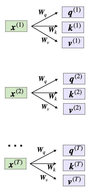
Here, both $q^{(i)}$ and $k^{(i)}$ are vectors of dimension $d_k$. The projection matrices $W_q$ and $W_k$ have shape $d × d_k$, while $W_v$ has shape $d × d_v$. Here $d$ denotes the number of dimensions of each word vector $x$, which is 3 in this article.

Because we need to compute the dot product of the query and key vectors, these two vectors must have the same number of elements ($d_q=d_k$). Many LLMs also use value vectors of the same size, that is, $d_q=d_k=d_v$. However, the number of elements in the value vector $v^{(i)}$ can be arbitrary; it determines the size of the resulting context vector.

In the code that follows, we set $d_q=d_k=2$ and $d_v=4$. The projection matrices are initialized as follows:

Input:

torch.manual_seed(123)

d = embedded_sentence.shape[1]

d_q, d_k, d_v = 2, 2, 4

W_query = torch.nn.Parameter(torch.rand(d, d_q))
W_key = torch.nn.Parameter(torch.rand(d, d_k))
W_value = torch.nn.Parameter(torch.rand(d, d_v))

In the original paper Attention Is All You Need, $d_q$, $d_k$, and $d_v$ are typically set to 64, while the total model dimension is 512.

Computing Unnormalized Attention Weights

In this section we walk through the computation using the second token as our example:

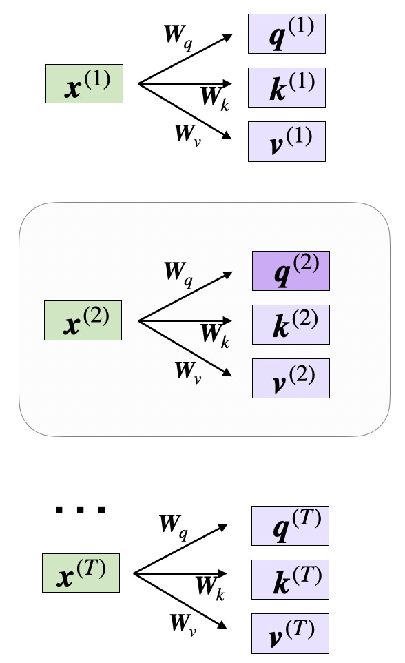
As the figure shows, we multiply the input $x$ by $W_q$, $W_k$, and $W_v$ respectively.

The code is as follows:

x_2 = embedded_sentence[1]
query_2 = x_2 @ W_query
key_2 = x_2 @ W_key
value_2 = x_2 @ W_value

print(query_2.shape)
print(key_2.shape)
print(value_2.shape)

Output:

torch.Size([2])
torch.Size([2])
torch.Size([4])

Generalizing, we can multiply embedded_sentence by $W_k$ and $W_v$ respectively; these results will be used in the following steps.

Input:

keys = embedded_sentence @ W_key
values = embedded_sentence @ W_value

print("keys.shape:", keys.shape)
print("values.shape:", values.shape)

Output:

keys.shape: torch.Size([6, 2])
values.shape: torch.Size([6, 4])

Now that we have $query^{(2)}$ along with all the keys and values, let us compute the unnormalized attention weights $\omega$, as shown below:

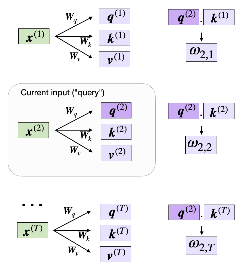
As the figure shows, $\omega (i,j)$ is the dot product between the query and key sequences: $\omega (i,j) = q^{(i)}k^{(j)}$.

For example, we can compute the unnormalized attention between the 2nd token’s query and the 5th token as follows:

Input:

omega_24 = query_2.dot(keys[4])
print(omega_24)

Output:

tensor(1.2903)

Generalizing, we can multiply query_2 by keys to obtain the unnormalized attention scores between the 2nd token and every other token.

Input:

omega_2 = query_2 @ keys.T
print(omega_2)

Output:

tensor([-0.6004,  3.4707, -1.5023,  0.4991,  1.2903, -1.3374])

Computing the Attention Weights

In the previous section we computed the unnormalized attention scores between the 2nd token and every other token. In practice, we also need to normalize these scores.

The purpose of normalization is to put the attention weight at each sequence position between 0 and 1, with all positions summing to 1. This probabilistic interpretation lets the model express, in probabilistic terms, how much attention it pays to different parts of the sequence: a higher weight means the model attends more to that position.

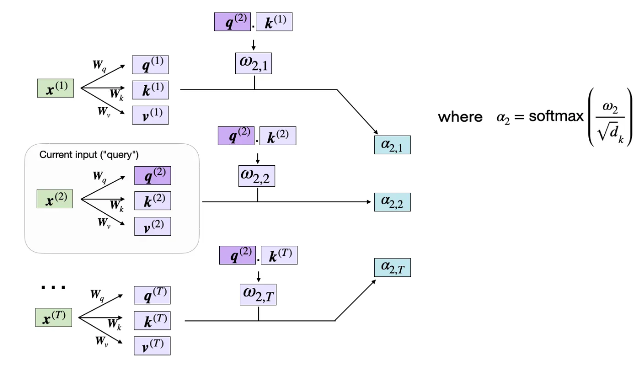
As the figure shows, self-attention first scales $\omega$ by $1/√{d_k} $ and then normalizes it with the softmax function.

Scaling by $d_k$ ensures that the Euclidean lengths of the weight vectors are all roughly on the same scale. This helps prevent the attention weights from becoming too small or too large — which could cause numerical instability or hurt the model’s ability to converge during training.

We can implement the attention weight computation in code like this:

Input:

import torch.nn.functional as F

attention_weights_2 = F.softmax(omega_2 / d_k**0.5, dim=0)
print(attention_weights_2)

Output:

tensor([0.0386, 0.6870, 0.0204, 0.0840, 0.1470, 0.0229])

The final step is to compute the context vector $z^{(2)}$ — an attention-weighted version of the original query input $x^{(2)}$ that incorporates all the other input elements as context through the attention weights:

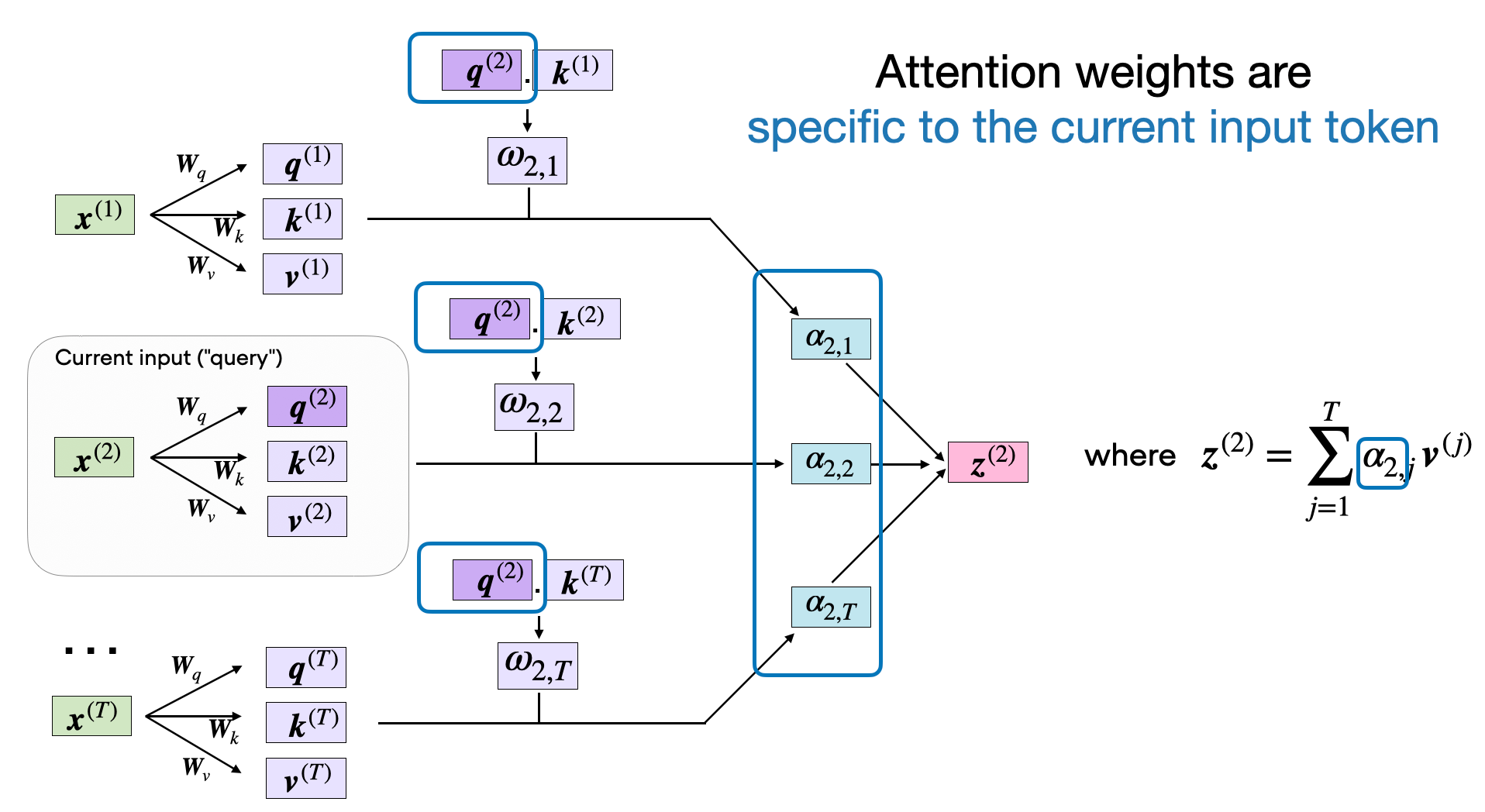
Input:

context_vector_2 = attention_weights_2 @ values

print(context_vector_2.shape)
print(context_vector_2)

Output:

torch.Size([4])
tensor([0.5313, 1.3607, 0.7891, 1.3110])

Note that this output vector has more dimensions ($d_v=4$) than the input vector ($d=3$), because we set $d_v > d$ earlier. The embedding size $d_v$, however, can be chosen arbitrarily.

Self-Attention

Now let us pull together the code for the self-attention mechanism from the previous sections.

We can condense everything above into a compact Self-Attention class:

import torch.nn as nn

class SelfAttention(nn.Module):

    def __init__(self, d_in, d_out_kq, d_out_v):
        super().__init__()
        self.d_out_kq = d_out_kq
        self.W_query = nn.Parameter(torch.rand(d_in, d_out_kq))
        self.W_key   = nn.Parameter(torch.rand(d_in, d_out_kq))
        self.W_value = nn.Parameter(torch.rand(d_in, d_out_v))

    def forward(self, x):
        keys = x @ self.W_key
        queries = x @ self.W_query
        values = x @ self.W_value

        attn_scores = queries @ keys.T  # unnormalized attention weights    
        attn_weights = torch.softmax(
            attn_scores / self.d_out_kq**0.5, dim=-1
        )

        context_vec = attn_weights @ values
        return context_vec

Input:

torch.manual_seed(123)

# reduce d_out_v from 4 to 1, because we have 4 heads
d_in, d_out_kq, d_out_v = 3, 2, 4

sa = SelfAttention(d_in, d_out_kq, d_out_v)
print(sa(embedded_sentence))

Output:

tensor([[-0.1564,  0.1028, -0.0763, -0.0764],
        [ 0.5313,  1.3607,  0.7891,  1.3110],
        [-0.3542, -0.1234, -0.2627, -0.3706],
        [ 0.0071,  0.3345,  0.0969,  0.1998],
        [ 0.1008,  0.4780,  0.2021,  0.3674],
        [-0.5296, -0.2799, -0.4107, -0.6006]], grad_fn=<MmBackward0>)

The second row is exactly the value of context_vector_2 from the previous section: tensor([0.5313, 1.3607, 0.7891, 1.3110]).

Conclusion

In this article we implemented self-attention by hand, with code and explanations, following Understanding and Coding Self-Attention, Multi-Head Attention, Cross-Attention, and Causal-Attention in LLMs.