Introduction

A refresher on the fundamentals

This article is part of my lecture notes from the Deep Learning Systems course taught by Tianqi Chen and J. Zico Kolter at CMU.

It covers the second lecture of the course: 2 - ML Refresher / Softmax Regression.

Defining the Data

In this section we define the input data used throughout this article.

Consider a $k$-class classification problem, in which we are given:

1. Training data: $x^{(i)}\in \mathbb{R}^n$, $y^{(i)}\in {1,…,k}$ $for$ $i = 1,..,m$.
2. n is the dimensionality of the input data
3. k is the number of classes/labels
4. m is the number of training examples

That completes the definition of all input data used in this article.

Linear Mapping

In this section we define the hypothesis function $h$ that maps the input data $x$ to $k$ classes.

We will use a linear function for this purpose, give its formal statement, and prove that the function is indeed linear.

Vector Form

Since we want to classify data $x$ of dimension $n$ into $k$ classes, we need to state this task formally.

For a $k$-class classification problem, we want to map an $n$-dimensional input vector $x\in \mathbb{R}^n$ into a $k$-dimensional solution space, that is $$ h{:}\mathbb{R}^n\to\mathbb{R}^k $$ where $h_i(x)$ denotes the confidence that the input $x$ belongs to class $i$.

This process can be expressed with a linear mapping function: $$ {h_\theta(x)=\theta^Tx} $$ where $\theta \in \mathbb{R}^{n\times k}$.

This completes the formal statement of the mapping function.

Why is $ h_\theta(x) = \theta^T x $ linear?

A linear function must satisfy additivity and homogeneity.

1. Additivity: Suppose we have two $n$-dimensional input vectors $x_1$ and $ x_2$. Then for the linear hypothesis function $h$ we have: $$ h_\theta(x_1 + x_2) = \theta^T (x_1 + x_2) $$ Since matrix multiplication is compatible with vector addition, by the distributive law: $$h_\theta(x_1 + x_2) = \theta^T x_1 + \theta^T x_2 $$ and the right-hand side equals transforming each vector separately and then summing: $$h_\theta(x_1 + x_2) = h_\theta(x_1) + h_\theta(x_2) $$ so additivity holds.

2. Homogeneity: If we take a scalar multiple $cx$ of $ x$, where $c$ is an arbitrary real number, the output of the linear hypothesis function $h$ is: $$ h_\theta(cx) = \theta^T (cx) $$ By the distributive law: $$ h_\theta(cx) = c(\theta^T x) $$ This shows that a scalar multiple transformed by ( h ) is exactly the transformation scaled by that scalar: $$ h_\theta(cx) = c h_\theta(x) $$

so homogeneity holds.

Matrix multiplication therefore satisfies both additivity and homogeneity, which proves that $h_\theta(x)$ is a linear function.

Matrix Form

In the previous subsection, $x$ was a vector of shape $1 \times n$. In this subsection we stack $m$ such vectors $x$ into a matrix of shape $m \times n$:

$$ X\in\mathbb{R}^{m\times n}=\begin{bmatrix}-{x^{(1)}}^T-\\\vdots\\-{x^{(m)}}^T-\end{bmatrix} $$

For a single vector $x$, its label $y$ is a real number. Likewise, when $m$ vectors $x$ are stacked into a matrix, the labels $y$ form a matrix of shape $m \times 1$:

$$ y\in\{1,...,k\}^m=\begin{bmatrix}y^{(1)}\\\vdots\\y^{(m)}\end{bmatrix} $$

Loss Functions

In this section we discuss the definitions, merits, and drawbacks of two loss functions — the 0-1 loss and the cross-entropy loss.

A loss function maps the model’s parameter matrix to a real number, and that number measures how good the hypothesis function $h_\theta(x)$ is.

0-1 Loss

For a classification problem, how do we judge whether a hypothesis function $h_\theta(x)$ is good?

A very intuitive idea is to assign $1$ when the prediction is wrong and $0$ when it is right. This is called the “0-1 loss function”. Its value depends on whether the classifier $h$’s prediction $h_\theta(x) $ on input $x $ matches the true label $y$. If the prediction is correct, the loss is 0; if it is wrong, the loss is 1. In short, the function asks only whether the classifier made a mistake, penalizing errors and nothing else. Formally:

$$ \ell_{err}(h(x),y)=\begin{cases}0&\text{if }\operatorname{argmax}_ih_i(x)=y\\1&\text{otherwise}\end{cases} $$

The advantage of this loss is its simplicity. Unfortunately, it is of little help when optimizing the model parameters, because it cannot be used with gradient-based methods — it has no gradient at all! When the prediction becomes correct, the loss jumps abruptly to 0, so there is no meaningful gradient direction to guide the parameter update.

Here, $ \text{argmax}_i h_i(x) $ denotes the class with the highest score among all the scores the classifier outputs.

Softmax and Cross-entropy Loss

The idea behind the “0-1 loss” of the previous subsection can be summed up as “all or nothing”: 1 for correct, 0 for wrong. Yet even among wrong answers, there is a difference between being slightly off and being wildly off.

With that in mind, we would like to turn the output of the hypothesis function $h_\theta(x)$ from a rigid all-or-nothing verdict into a “probability”. Here we can use the softmax function, which converts any vector of real numbers into a probability distribution. For class $i $, the probability predicted by the model, $p(\text{label} = i) $, is computed as the exponential of that class’s score $ h_i(x) $ divided by the sum of the exponentials of all class scores, which ensures that the predicted probabilities sum to 1. Formally:

$$ z_i=p(\text{label}=i)=\frac{\exp\bigl(h_i(x)\bigr)}{\sum_{j=1}^k\exp\bigl(h_j(x)\bigr)}\Longleftrightarrow z\equiv\text{softmax}\bigl(h(x)\bigr) $$

Dividing the output by the sum of all outputs is easy to understand: normalizing this way makes every class output fall between 0 and 1 and makes the outputs sum to 1. The less obvious part is why we exponentiate $ h_i(x) $ in the first place.

There are two main reasons:

1. Exponentiating turns the hypothesis function’s outputs into positive values. This is necessary for a valid probability distribution, since probabilities cannot be negative.
2. The exponential curve is increasing, and — most importantly — its slope grows steadily, meaning that a small change along the x-axis can produce a large change along the y-axis. This helps sharply distinguish the classes with higher raw logits when computing probabilities.

With the softmax function in hand, we can compute the loss with the cross-entropy loss, stated formally as:

$$ \ell_{ce}(h(x),y)=-\log p(\text{label}=y)=-h_y(x)+\log\sum_{j=1}^k\exp\left(h_j(x)\right) $$

Note that the cross-entropy loss is essentially the $-log$ of the softmax output for class $y$.

Adding the $log$ serves two purposes:

1. It maps values in the interval (0, 1) to the interval from negative infinity to 0, so that small changes in probability are amplified in the loss value, providing better discrimination.

2. When the predicted probability is close to that of the true label, the gradient of the loss becomes small and the model learns more slowly. Conversely, when the prediction differs greatly from the true label, the gradient becomes markedly larger and the model learns faster. This lets the model learn more effectively, adjusting course quickly when it frequently makes wrong predictions.

Adding the $-$ turns negative values into positive ones, so that a larger discrepancy means a larger loss, and vice versa.

Optimization

As noted above, the loss function lets us judge how good the weight parameters of the hypothesis function $h_\theta(x)$ are.

So if the weights in $h_\theta(x)$ are not good enough, how should we optimize them?

Definition

Broadly speaking, we want to optimize the weight parameters $\theta$ so as to minimize the output of the loss function. Formally: $$ \underset{\theta}{\operatorname*{minimize}}\frac1m\underset{i=1}{\operatorname*{\sum}}\ell(h_\theta(x^{(i)}),y^{(i)}) $$ where $i$ is the index of the current sample, $h$ is the hypothesis function, and $y$ is the sample’s true label (ground truth).

Substituting the cross-entropy loss $\ell_{ce}$ for $\ell$ gives: $$ \underset{\theta}{\operatorname*{minimize}}\frac1m\sum_{i=1}^m\ell_{ce}(\theta^Tx^{(i)},y^{(i)}) $$ That gives us the definition of the optimization problem.

Concretely, then, how do we carry out the optimization?

Gradient-based Optimization

Gradients

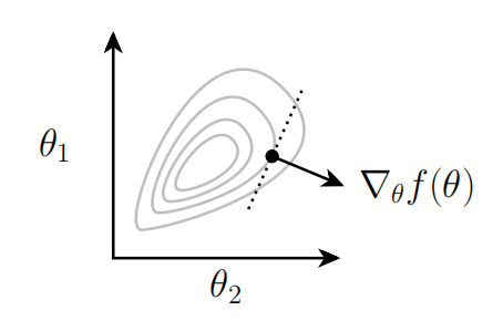
For a function $f{:\mathbb{R}^{n\times k}\to\mathbb{R}}$ that takes a matrix as input and returns a real number, its gradient is defined as the matrix of partial derivatives, stated formally as:

$$ \nabla_\theta f(\theta)\in\mathbb{R}^{n\times k}=\begin{bmatrix}\dfrac{\partial f(\theta)}{\partial\theta_{11}}&...&\dfrac{\partial f(\theta)}{\partial\theta_{1k}}\\\vdots&\ddots&\vdots\\\dfrac{\partial f(\theta)}{\partial\theta_{n1}}&...&\dfrac{\partial f(\theta)}{\partial\theta_{nk}}\end{bmatrix} $$

Combining this with the discussion above, $f$ here stands for the loss function.

Mathematically, the gradient points in the direction of steepest local ascent of the loss function.

In optimization, therefore, we adjust the parameters along the negative gradient in order to minimize the loss.

Learning Rate

Armed with the gradient, a powerful tool, we can now update the weight parameters.

Note, however, that we update the weights round by round. We therefore need a scaling factor $\alpha$ that defines how much the weights are updated in each round of training. This scaling factor $\alpha$ is called the learning rate. When updating weights with the gradient, each step can be stated formally as: $$ \begin{aligned}\theta:=\theta-\alpha\nabla_\theta f(\theta)\end{aligned} $$ where:

• $\theta$ is the weight parameter to be optimized.
• $\alpha$ is the learning rate, a positive number controlling the size of each update step.
• $\nabla_\theta f(\theta)$ is the gradient of the loss function $f(\theta) $ with respect to the parameter $ \theta$.

This method is the well-known Gradient Descent. It works by computing the gradient of the loss function at the current parameters, then updating the parameters along the negative gradient direction, iterating until convergence.

In gradient descent, choosing an appropriate learning rate is crucial to optimization performance. The three subplots below show the paths taken by gradient descent in a two-dimensional parameter space under different learning rates $\alpha$, where the contour lines represent the value of the loss function. From left to right, the learning rates are 0.05, 0.2, and 0.42. The goal of gradient descent is to find the global minimum of the loss function, which is the innermost contour ring in the figure.

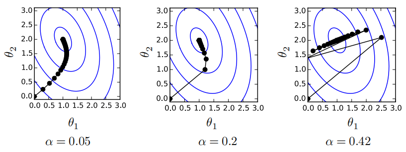
From these three subplots we can observe that:

• When the learning rate is small (0.05, left), the descent path is long and many more iterations are needed to reach the minimum. This means we must run many rounds of iteration before finding the optimal weights.
• When the learning rate is moderate (0.2, middle), gradient descent approaches the minimum fairly quickly.
• When the learning rate is large (0.42, right), the updates may overshoot, causing the descent path to wander around the minimum and struggle to settle down.

We therefore need to choose the learning rate carefully. The reasons are:

• Convergence speed: if the learning rate is too small, gradient descent may converge to the minimum very slowly, increasing the number of iterations needed to reach the optimum and making training take much longer.
• Oscillation: if the learning rate is too large, the parameter updates may overshoot, causing the algorithm to jump around the minimum or even past it, so that the loss actually increases. This makes the algorithm diverge and never find the minimum.
• Avoiding poor local minima: a well-chosen learning rate can help the algorithm converge accurately to the global minimum of the loss function, or to a good local minimum, rather than to a mediocre local minimum or a saddle point.
• Stability: an overly large learning rate can cause oscillation around the minimum instead of convergence, whereas an appropriate learning rate ensures that the parameter updates approach the optimum smoothly and stably.

Stochastic Gradient Descent

The previous subsection introduced gradient descent, giving us a paradigm for optimizing weight parameters. In practice, however, we more often update weights using an optimization method called Stochastic Gradient Descent (SGD).

In machine learning, when the loss function is a sum of individual losses, we would rather not compute the gradient over all samples just to perform a single parameter update, because that is expensive in both computation and time.

Instead, we can take only a small portion of the dataset (called a minibatch) at a time to compute the gradient and update the parameters. This uses fewer computational resources and lets us make many more parameter updates in the same amount of time.

We define a minibatch formally as: $$ X\in\mathbb{R}^{B\times n},y\in{1,…,k}^B $$

The stochastic gradient descent update can then be expressed formally as: $$ \theta:=\theta-\frac{\alpha}{B}\sum_{i=1}^{B}\nabla_{\theta}\ell(h_{\theta}(x^{(i)}),y^{(i)}) $$

Computing the Gradient of the Cross-entropy Loss

In the previous section we learned how to use gradients to update the weight parameters. We are now just one step away from our goal — computing the gradient.

So how do we compute the gradient of the cross-entropy loss? $$ \nabla_\theta\ell_{ce}(\theta^Tx,y)=? $$ By the chain rule, the expression above can be written as: $$ \frac\partial{\partial\theta}\ell_{ce}(\theta^Tx,y) = \frac{\partial\ell_{ce}(\theta^Tx,y)}{\partial\theta^Tx}\frac{\partial\theta^Tx}{\partial\theta} $$ The right-hand side splits into two terms, namely: $$ \frac{\partial\ell_{ce}(\theta^Tx,y)}{\partial\theta^Tx} \tag{1} $$ and $$ \frac{\partial\theta^Tx}{\partial\theta} \tag{2} $$ For ${(1)}$:

Remember the formula for the cross-entropy loss? Let us take the partial derivative of the loss with respect to the output $h_i$ of some class.

$$ \begin{aligned} \begin{aligned}\frac{\partial\ell_{ce}(h,y)}{\partial h_i}\end{aligned}& \begin{aligned}=\frac{\partial}{\partial h_i}\left(-h_y+\log\sum_{j=1}^k\exp h_j\right)\end{aligned} \\ &=-1\{i=y\}+\frac{\exp h_i}{\sum_{j=1}^k\exp h_j} \end{aligned} $$

Here we make a surprising discovery: the derivative of the cross-entropy loss contains $\frac{\exp h_i}{\sum_{j=1}^k\exp h_j}$! Looks familiar, doesn’t it? That is exactly the expansion of Softmax(h(x))!

We can therefore simplify the result above to $\begin{aligned}\nabla_h\ell_{ce}(h,y)=z-e_y\end{aligned}$, where $z=\mathrm{softmax}(h)$ and $e_y$ is the one-hot vector corresponding to the correct class.

For ${(2)}$:

The derivative is easy to obtain: $$ \frac{\partial\theta^Tx}{\partial\theta} = x $$ So equation $(0)$ can be expressed as:

$$ \begin{aligned} \begin{aligned}\frac{\partial}{\partial\theta}\ell_{ce}(\theta^Tx,y)\end{aligned}& \begin{aligned}=\frac{\partial\ell_{ce}(\theta^Tx,y)}{\partial\theta^Tx}\frac{\partial\theta^Tx}{\partial\theta}\end{aligned} \\ &=({z-e_y})(x),\quad\text{where }z=\text{softmax}(\theta^Tx) \end{aligned} $$

Just one more step to go!

Let us do a little more work to align the matrix shapes…

So, when the input is a vector $x$, the gradient of the cross-entropy loss with respect to the weight matrix $\theta$ is: $$ \nabla_\theta\ell_{ce}(\theta^Tx,y)\in\mathbb{R}^{n\times k}=x(z-e_y)^T $$ Extending the input to the matrix $X$ formed by stacking all vectors $x$ in a batch, the expression becomes: $$ \nabla_\theta \ell_{ce}(X\theta, y) \in \mathbb{R}^{n \times k} = X^T(Z - I_y) $$ where:

• $X$ is the feature matrix of the entire data batch.
• $Z$ is the matrix of predicted probabilities produced by the hypothesis function for the whole batch. Each row is the predicted probability distribution of one sample, obtained by passing $X\theta$ through the softmax function.
• $ I_y $ is a matrix in which each row is the one-hot vector of the correct class for one sample.

With that, we have completed the gradient computation for the cross-entropy loss, and we can use the gradient to update the weight matrix!

Conclusion

In this article we covered the softmax function, the cross-entropy loss, gradients, gradient descent, stochastic gradient descent, and how to use gradient descent to optimize weight parameters.

Stay tuned for the follow-up articles!