Preface

Working on LLM-enhanced graph problems lately has given me an interest in heuristic algorithms on graphs, and a quick search turned up this survey from 2006. The paper is old, but shortest path algorithms have not been a hot research area over the past two decades, so there is little newer work to read; besides, many recent papers on LLM reasoning take their inspiration from classical algorithms. Here, then, is my summary of it.

Introduction

Although standard optimal shortest path algorithms can already solve most shortest path problems, they often fail to meet the requirements of tasks on large-scale graphs with low latency. In an in-vehicle route guidance system, for example, an immediate response is required. In such tasks the result does not necessarily have to be “optimal” — “good enough” will do. Heuristic shortest path algorithms were born of this need.

Over the past six decades, researchers have proposed many heuristic methods for reducing the computation time of shortest path algorithms. This paper reviews the various heuristic shortest path algorithms developed over that period.

The Shortest Path Problem and Optimal Algorithms

Let the directed graph be $G(N,A)$, with $N$ vertices and $A$ directed edges. Let $n = |N|$ denote the number of vertices and $m = |A|$ the number of edges. Let $a=(i,j)\in A$ denote a directed edge from $i$ to $j$, and $c_{i,j}$ the cost of going from $i$ to $j$. A path from origin $o$ to destination $d$ can be defined as $path = (o,j),\ldots,(i,d)$, and its cost is the sum of the costs of all its edges, $cost_{path} = \sum_{(i,j)\in path} c_{i,j}$. The shortest path problem is to find the path that minimizes $cost$, $path = {\arg \min}_{path \in \text{all paths}} (cost_{path})$.

Optimal Algorithms

The shortest path problem (SPP) has been studied for more than 40 years in fields such as computer science and transportation. Because of their computational tractability, most research in this area has focused on developing increasingly efficient optimal algorithms for the problem. Most optimal shortest path algorithms are essentially applications of dynamic programming theory to searching for shortest paths in a graph. The shortest path is found through a recursive decision process from the source node to the destination node.

Most shortest path algorithms follow a standard procedure like the one below:

1. Initialization:

   $\begin{array}{l}i=o;L_{(i)}=0;L_{(j)}=\infty;\forall j\neq i;P_{(i)}=\text{NULL.}\\Q=\{i\};\end{array}$

2. Node selection:

   Select node $i$ and remove it from $Q$.

3. Node expansion

   Scan the edges emanating from $i$. For an edge $\alpha=(i,j)$, if $L_{(i)}+c_{a}<L_{(j)}$ then $L_{(j)}=L_{(i)}+c_{a};P_{(j)}=a$ and insert $j$ into the set $Q$.

4. Termination check

   If $Q = \emptyset $, stop; otherwise, repeat Step 2.

Here, the cost from the origin node $o$ to node $i$ is denoted $L(i)$; $P$ is the list that stores, for each node, the incoming edge on the shortest path tree, so $P(i)$ is the incoming edge on the shortest path to node $i$; and $Q$ is the set of nodes to be scanned, which manages the nodes to be examined during the search.

Label-setting algorithm (LS)

The elements of $Q$ are sorted by their current cost.

One notable feature of this approach is that if only the path from the origin node to a single destination node is needed, the algorithm can terminate as soon as the cost of the destination node has been computed. This mode of operation is usually called a one-to-one search pattern.

Dijkstra’s algorithm is an example.

Label-correcting algorithm (LC)

The elements of $Q$ are filled and scanned while the shortest path tree is being built.

Its defining feature is that it cannot report the shortest path between two nodes until the shortest paths to every node in the network have been determined, a mode of operation known as a one-to-many search pattern.

Bellman-Ford and SPFA are examples.

Computational Performance

Among LC algorithms, the double-ended queue and the threshold list data structures dominate in terms of computational efficiency.

Among LS algorithms, Dial’s bucket implementation and the binary heap data structure are the most efficient.

Heuristic Shortest Path Algorithms

For real-time problems in practice, the optimal shortest path algorithms discussed above are often far too computationally expensive.

This “inefficiency” stems from the fact that these algorithms employ “uninformed” outward search techniques that make no use of prior knowledge about the locations of the origin and destination nodes, the composition of the path, or the structure of the network.

For instance, if the origin node lies in the city center and the destination node lies in the south of the city, an optimal algorithm is just as likely to search for minimum-cost routes north of the origin node as south of it.

Intuitively, the more information the search uses, the more efficient the algorithm can be. Researchers in AI recognized this early on and proposed many heuristics that attempt to reduce the search effort by drawing on additional sources of knowledge.

Heuristic search strategies can generally be divided into four kinds:

1. Limit the search area
2. Decompose the search problem
3. Limit the links searched
4. Some combination of the above

Next we examine these heuristic search strategies and their application to shortest path search.

Limiting the Search Area

The idea behind the “limit the search area” strategy is to draw on prior knowledge about the shortest path from the origin node to the destination node to confine the search to a certain region.

The resulting search area is much smaller than that of an optimal algorithm operating without prior knowledge.

Pruning

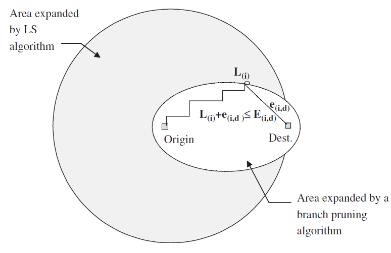
The basic idea here is to limit the search area by “pruning” those intermediate nodes that are very unlikely to lie on the shortest path to the destination node.

In a classical urban transportation network, each link (or road segment) is normally connected only to adjacent nodes (such as intersections), and the travel time on a link usually correlates with its length. This property allows the search area to be confined to a designated region around the origin and destination nodes. Nodes outside this region are assumed to have a small probability of lying on the shortest path and can therefore be excluded during the search without further examination.

The key is to define the search area in a way that effectively reduces computation time while still yielding a good solution.

Some researchers have proposed constraining the search range with the following inequality: $$ L_{(i)}+e_{(i,d)}\leqslant E_{(o,d)}, $$ where $L(i)$ is the current minimum cost from the origin node $o$ to node $i$; $e(i,d)$ is the estimated cost from node $i$ to the destination node $d$; and $E(o,d)$ is an upper bound on the minimum cost from the origin node to the destination node.

Incorporating this method into the optimal LC algorithm requires only a modification to Step 2:

2. Select node $i$ and remove it from $Q$. If $L_{(i)}+e_{(i,d)}\leqslant E_{(o,d)}$, jump to Step 4.

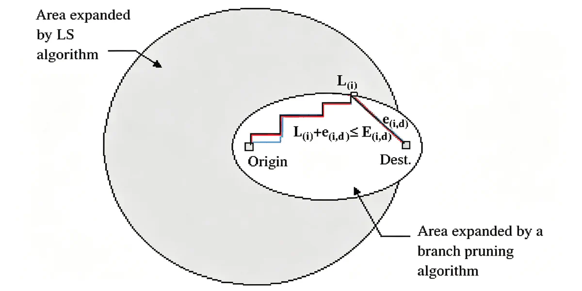
The efficiency of the branch-pruning algorithm is illustrated in the figure above. The new heuristic strategy shrinks the search area from the circle expanded by the optimal LS algorithm to an ellipse. On an ideal Euclidean grid, the search area of such heuristic algorithms can be as small as 20% of that of the LS algorithm.

The efficiency and accuracy of a branch-pruning shortest path algorithm depend on the quality of the estimation functions $e(i,d)$ and $E(o,d)$. Optimality is clearly preserved only when $e(i,d)$ always stays below the minimum cost from node $i$ to the destination node $d$ while $E(o,d)$ always stays above the minimum cost from the origin node $o$ to the destination node $d$. It is also worth noting that as $e(i,d)$ approaches zero and $E(o,d)$ approaches infinity, the branch-pruning algorithm degenerates into an optimal shortest path algorithm.

In short, with the method above, $e$ should be underestimated and $E$ overestimated.

A*

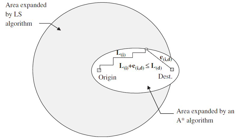
In the pruning approach, nodes with a low probability of lying on the shortest path are pruned away. The A* algorithm instead keeps these nodes in $Q$ but assigns them a low priority.

A* uses a heuristic evaluation function $F_{(i)}=L_{(i)}+e_{(i,d)}$ as the label of node $i$, where $L(i)$ is the cost of the currently evaluated path from the origin node to node $i$ and $e(i,d)$ is the estimated cost from node $i$ to the destination node $d$. The sum $F$ of the two functions reflects the likelihood that $i$ lies on the shortest path: the lower $F$ is, the more likely $i$ is to appear on the shortest path. Building on this idea, the algorithm performs a best-first search: it maintains a list $Q$ of nodes to be scanned, sorted by their $F$ values, and selects the node with the lowest $F$ value for expansion. The selected node is expanded by visiting its neighbors, which are then inserted into $Q$ in order according to their $F$ values. This process continues until the destination node is selected for expansion. A* therefore bears a resemblance to the LS algorithm.

Here is a recommended article for understanding A*; it is clearly organized and offers interactive pages: https://www.redblobgames.com/pathfinding/a-star/introduction.html

Compared with the LS algorithm, A* uses the evaluation function $F(i)$ rather than $L(i)$ to determine the order of nodes in $Q$.

The main difference lies in Step 3, modified as follows:

3. Node expansion

   Scan the edges emanating from $i$. For an edge $\alpha=(i,j)$, if

   $L_{(i)}+c_{ij}+e_{(j,d)}<F_{(j)},$

   then

   $\begin{array}{l}L_{(j)}=L_{(i)}+c_{ij};F_{(j)}=L_{(i)}+c_{ij}+e_{(i,d)};P_{(j)}=a,\end{array}$

   and insert $j$ into the set $Q$.

Because A* is based on the best-first idea, any node satisfying the following inequality will be scanned before the algorithm terminates: $$ L_{(i)}+e_{(i,d)}\leqslant L_{(d)}. $$ Hence, as long as the estimation function never overestimates the cost, the optimal solution can be found.

Decomposing the Search Problem

It is widely recognized that the amount of computation required to solve a general search problem usually grows faster than the size of the problem itself. For example, the computation time needed to find the shortest path from an origin node to a destination node depends on the number of nodes searched before the destination is reached, so the computational effort is a higher-order polynomial function of distance. Consequently, decomposing the original problem into smaller subproblems can dramatically reduce complexity.

This section describes how to realize this strategy using bidirectional search and the subgoal method.

Bidirectional Search Strategy

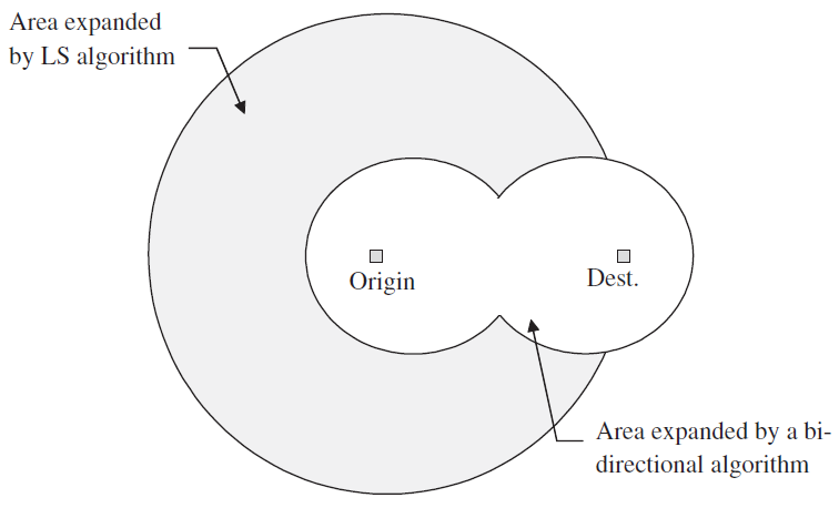
The bidirectional search strategy attempts to split the search process into two independent processes: one advancing forward from the origin, the other working backward from the destination. When these two search processes meet at some intermediate stage, the solution is found.

As the figure above shows, the algorithm builds shortest path trees outward from the origin and the destination simultaneously, until some stopping condition is met.

The effectiveness of a bidirectional algorithm is influenced by two factors:

1. The rule for alternating between the forward and backward searches.
2. When the algorithm stops.

For the former, the most intuitive approach is to alternate evenly. Even alternation, however, is not necessarily the most efficient. The best strategy should find the shortest path while scanning as few nodes as possible.

For the latter, some researchers have proposed the following condition: $$ L_{(i)}^o+L_{(i)}^d\leqslant\min_{j\in N}{L_{(j)}^o}+\min_{j\in N}{L_{(j)}^d} $$ What this expression captures is that, for any node $j$, the minimum cost from $o$ to $j$ plus the minimum cost from $j$ to $d$ is greater than or equal to the shortest distance from $o$ to $d$ passing through $i$. In that case, $i$ must be a node on the shortest path from $o$ to $d$.

The astute reader will quickly notice, however, that this is a rather poor criterion.

Sure enough, researchers have shown that with this stopping criterion the resulting bidirectional search algorithm performs worse than a unidirectional one. It is conjectured that the nodes expanded by the bidirectional search process may grow into almost complete unidirectional trees before the condition is satisfied, rather than meeting “in the middle” between the origin and the destination.

A number of researchers later proposed improvements on this basis, such as bidirectional A* with a modified estimation function, or bidirectional A* using multiple intermediate meeting nodes.

The Subgoal Method

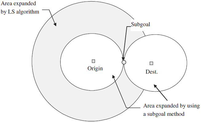
A subgoal can be defined as an intermediate state of the optimal solution to a problem. For shortest path search in a road transportation network, subgoals may be those nodes or links located between the origin and the destination, between which the shortest path needs to be determined. If the location of a subgoal is known in advance, the problem of finding the shortest path from origin to destination can be decomposed into two or more smaller problems.

For example, given a single subgoal node, the original problem can be solved by solving two subproblems: finding the shortest path from the origin to the subgoal node, and finding the shortest path from the subgoal node to the destination.

If a subgoal node is known and lies midway along the shortest path from the origin to the destination, using it will reduce the search area by roughly 50% compared with the LS algorithm, as shown in the figure above. If one of the techniques for limiting the search area is used at the same time, the computational savings will be even greater.

The reason this method works is that if we know $i$ to be an intermediate node on the shortest path from $o$ to $d$, then the cost of the shortest path from $o$ to $d$ must equal the cost of the shortest path from $o$ to $i$ plus the cost of the shortest path from $i$ to $d$.

Limiting the Links Searched

During shortest path search, the main decision at each iteration concerns which edges emanating from each node to scan. In traditional shortest path algorithms, when a node is selected for expansion, all edges out of that node are scanned, no matter how likely they are to lie on the shortest path.

The basic idea of limiting the links searched is to skip edges that have a low probability of lying on the shortest path or of being used in practice. The hierarchical search method discussed in the next section is an effective way to implement it.

Hierarchical Search

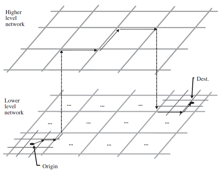
The basic idea behind hierarchical search is that to solve a complex problem efficiently, the search process should first concentrate on the essential features of the problem, ignoring lower-level details, and only then fill those details in.

Take a driver looking for a route between two locations: we first find the arterial roads the route requires, and then find the minor roads connecting those arterials. The first step narrows the search to arterial roads alone, and the second narrows it to the minor roads attached to them.

Two questions must be resolved for this method:

1. How should real-world roads be mapped into a hierarchical graph?
2. How should transitions between levels be controlled? When should the search switch to the next level?

Freeways and major traffic arteries are designed for long-distance travel, whereas local streets mainly serve local vehicle trips. Road links can therefore conveniently be classified according to their function. Some researchers have proposed using edge length as the criterion, extracting long edges to form the high-level subnetwork and grouping shorter edges and their nodes into the low-level subnetwork. Others have proposed dividing all roads into two levels based on attributes such as speed limit and number of lanes.

One problem with hierarchical search algorithms is that they cannot take shortcuts between two arterial roads — moving from one arterial to another via residential streets, for instance. These algorithms are designed to simplify the search by classifying roads into levels (freeways, arterials, residential streets, and so on) and thereby reducing the number of roads that must be considered, and they usually consider higher-level roads such as freeways before lower-level ones such as residential streets.

Reference

Title: Heuristic shortest path algorithms for transportation applications: State of the art

Institution: University of Waterloo, Chongqing University, University of Nebraska-Lincoln

Authors: L. Fua, D. Sunb, L.R. Rilettc

DOI: https://doi.org/10.1016/j.cor.2005.03.027

Date: 2006.11.01