Preface
These are my notes from the workshop given by Google’s Graph Mining Team at NIPS 2020.
The project homepage is Graph Mining & Learning, and the PDF version is available at Mining and Learning with Graphs at Scale.
Introduction
What Is a Graph?
A graph is a form of data that represents relationships between entities.
Here, an entity corresponds to a node, and a relationship corresponds to an edge.
In general, graphs have the following characteristics:
- A large number of edges
- Multiple types of edges and multiple types of nodes
- Highly complex structure
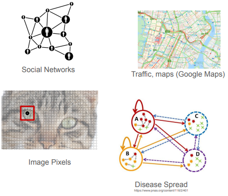
Graphs can therefore be used to represent social networks, transportation networks, and much more.
Types of Graphs
Broadly speaking, graphs fall into two categories: natural graphs and similarity graphs.
Natural Graphs
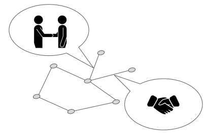
In a natural graph, the edges come from external, real-world circumstances or data. In other words, the entities and relationships the graph represents genuinely exist in the real world. For example, every transaction in a payment network can be seen as an edge linking the payer and the payee; in a social network, a friendship between two people can likewise be expressed as an edge; in a road network, roads connect different locations; and in co-click or co-watch data, if two items are clicked or watched by the same person, an edge can be drawn between them. What defines this kind of graph is that the existence and nature of its edges are determined by real-world relationships or interactions.
Similarity Graphs
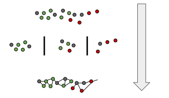
In contrast to natural graphs, the edges of a similarity graph come from the similarity between nodes. Here we start with a large collection of metadata or data and then build the graph structure by measuring the similarity or distance between data points. For instance, given a set of articles, we can connect them based on the similarity of their content (say, keyword overlap or topical similarity) to form a graph. In this case, edges are created by analyzing and computing over the properties of the data itself, rather than being derived from relationships that already exist externally.
Note: when working with similarity graphs, the original metadata of each node remains available to us. For high-dimensional metadata, preprocessing and precomputation can avoid a great deal of redundant computation and therefore save considerable time.
Why Use Graphs?
Computation on Abstract Concepts
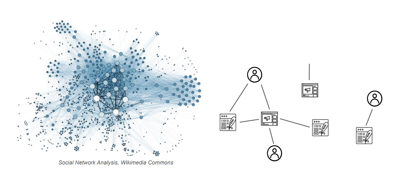
“Computation on abstract concepts” means handling complex relationships with graphs. Interpersonal ties in a social network, route connections in a transportation system, and causal relationships in scientific research are all typically complicated, yet much of this data can be reduced to interactions and connections among entities — that is, to a graph. Graphs are a powerful tool for understanding and manipulating such relationships. They help us not only understand and analyze local information (between directly connected entities) but also abstract over that information, extracting general patterns or principles from specific instances and local situations. Abstracting local information this way lets us pull useful global information out of the data as a whole: identifying key nodes across an entire network (opinion leaders in a social network, say), discovering group structure through community detection, or understanding how the overall structure shapes individual behavior and system performance.
Computation on Multimodal Data
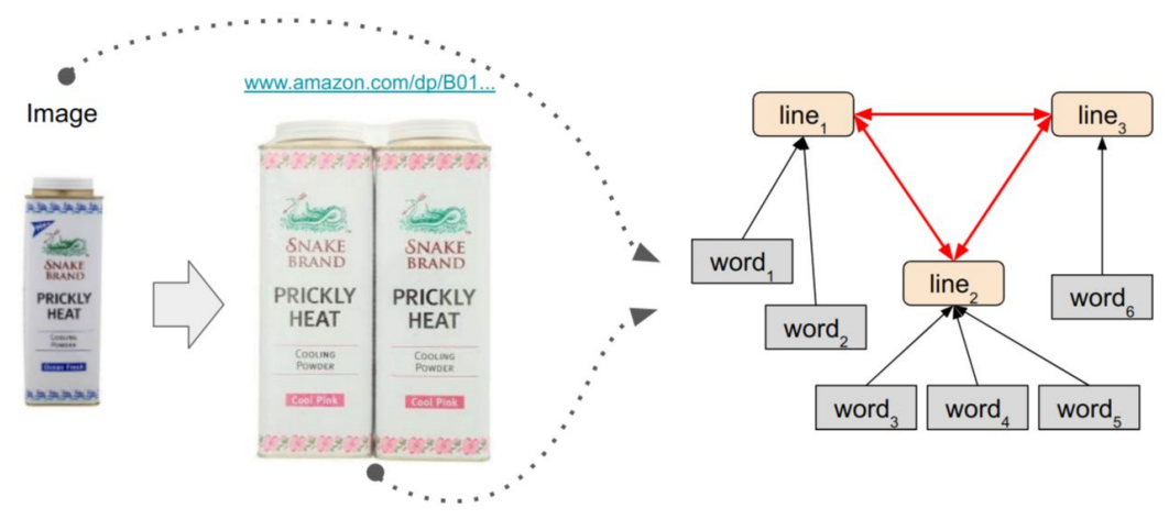
In many scenarios we have to handle data of several modalities at once — visual, textual, semantic information — and these data are interrelated. Graphs let us relate data across modalities and compute over them jointly.
The Global View
Graph structure can help us discover patterns, groups, or relationships in data, and can even quantify concepts that are intrinsically hard to measure directly.
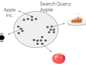
Take the figure above as an example: given an ambiguous picture of an apple, we can compute its similarity to a cluster of Apple Inc. images and to a cluster of natural apple images, and thereby determine which cluster the picture belongs to.
The Local View
By computing over graph structure, a graph can supply information that goes beyond the attributes of any single node. Concretely, a node on its own tells us only so much; but by computing over the nodes and edges around it, we can learn a great deal more.
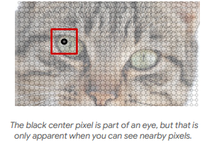
Take the figure above as an example: looking at a single pixel, we have no idea what it means. But by looking at the pixels around it, we can tell that the pixel comes from a cat’s eye.
The Graph Mining Toolbox
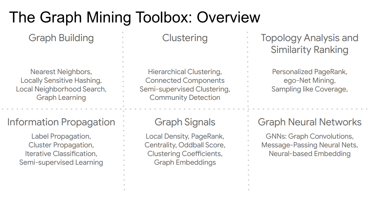
This part of the talk introduces the toolbox developed and used by Google’s Graph Mining Team. Since it comes up again later, we skip the details here.
Application Cases
Spam, Fraud, and Abuse Detection
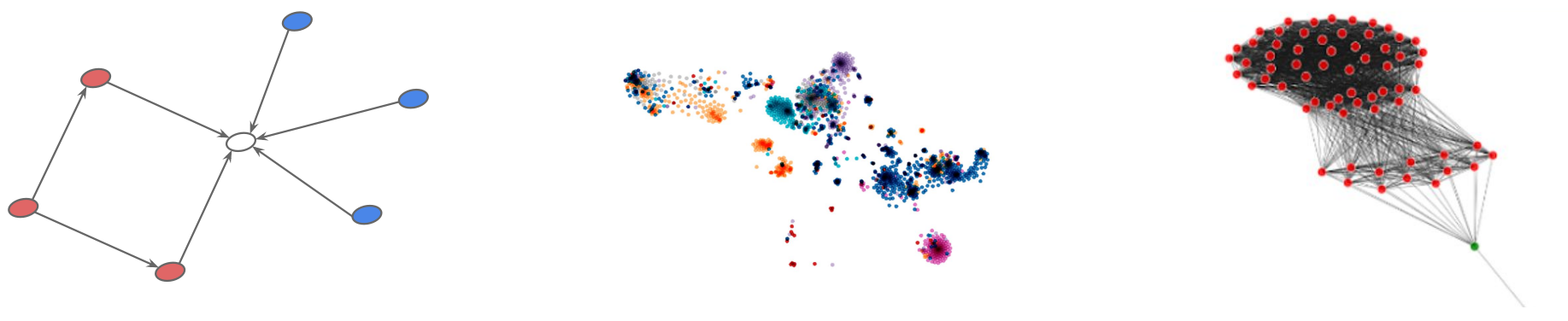
For detecting spam, fraud, and abuse — particularly in trust and safety work — the Google team presents two core ideas and methods: anomaly detection via density clustering, and label propagation.
Anomaly detection via density clustering:
Statistically improbable dense clusters correlate strongly with malicious behavior. In other words, if we find unusually dense clusters of nodes in a graph representation of the data, those clusters very likely correspond to spammers, fraud, or other kinds of abuse. Graph mining tools can identify these unusual dense clusters and thus detect and prevent malicious behavior. This is essential for keeping products such as YouTube and the ad platforms safe and trustworthy.
Label propagation:
Starting from known bad actors, we use the graph structure to identify neighboring nodes that are likely problematic as well. The intuition is that malicious users or entities tend to sit close to one another in the graph or to be connected in some way — for example, they may jointly participate in fraud or spam campaigns. By propagating a label (such as “malicious”) from known bad actors to the nodes they connect to, we can surface additional suspicious actors. This effectively broadens the detection net and uncovers entities that were never directly flagged as malicious.
Improving Machine Learning Models
Relationship discovery:
The way social networks find “people you may know” is by analyzing the social graph. Graph information can reveal non-obvious connections: even when a link is not apparent from direct social interaction, graph analysis can expose latent ties such as mutual friends, shared interests, or similar social paths.
Feature extraction:
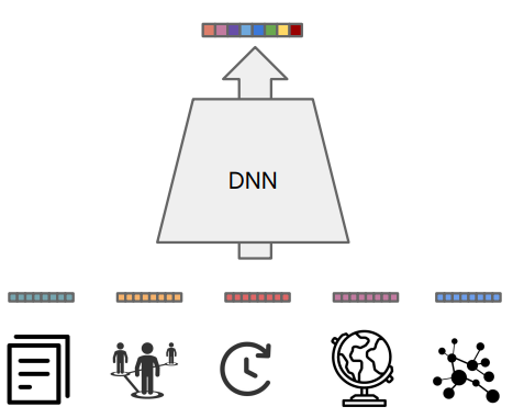
Signals produced from graphs — clusters, personalized PageRank (PPR) vectors, and graph embeddings — are highly useful for training downstream machine learning models. These graph-derived features can substantially improve model performance by providing deep information about relationships between entities. In multimodal models, graph data can serve as yet another modality, joining text, images, and audio to form a larger whole. This lets machine learning models draw on a richer dataset and thereby achieve a more comprehensive understanding and more accurate predictions.
A case study:
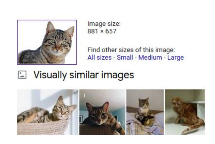
Consider the “visually similar images” feature of Google Images. By analyzing similarity between images, one can build a graph in which nodes are images and edges represent visual similarity. Even when a user specifies no explicit search criteria, the system can find other images that are visually similar to a given one.
Efficient Computation
Resource efficiency: communication overhead
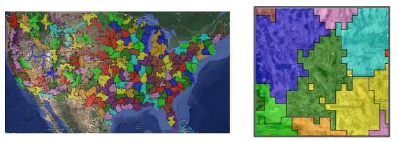
In distributed computing systems, large datasets must be partitioned and spread across compute nodes, and the resulting communication overhead can be reduced with graph partitioning algorithms. Applying graph partitioning in Google Driving Directions, for instance, optimizes backend processing and makes road network data processing far more efficient.
Data efficiency and active learning
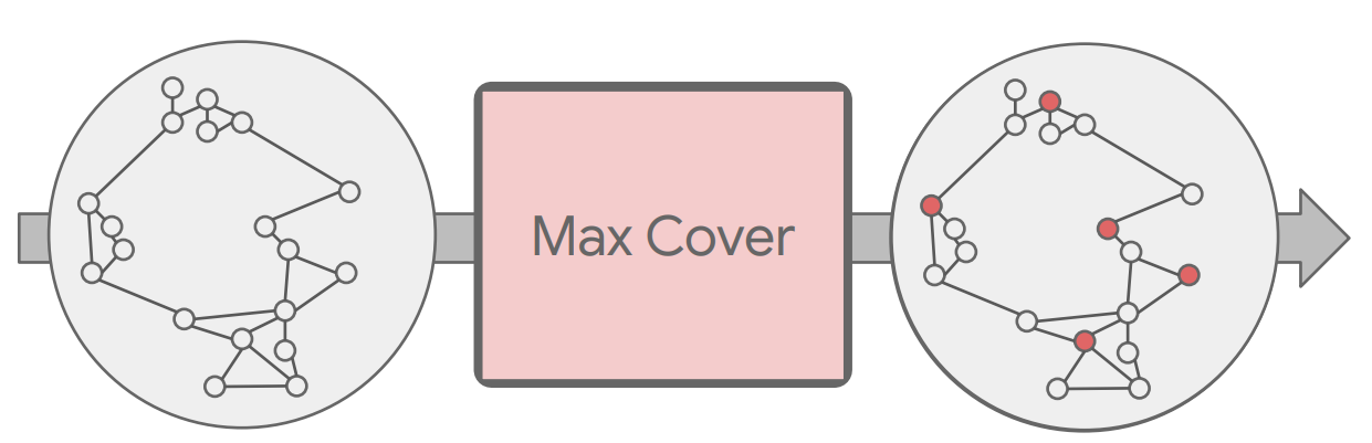
Graphs let us answer queries such as “which points in my dataset are the most diverse,” which can drive an active learning loop. Active learning is a strategy that allows a model to request annotations for specific data points so as to learn and improve as efficiently as possible; it is especially suited to settings where labeled data is scarce. Graph-based semi-supervised learning suits models with little data: it can leverage a small amount of labeled data together with a large amount of unlabeled data, using graph structure to improve learning.
Application Stories
Modeling COVID Spread with Spatio-Temporal Graph Neural Networks
Fundamentals
A deep machine learning model can be described as learning a function $f(x)$, where $x$ is a carefully chosen set of features. The model’s intermediate states — the embeddings — capture the complex interactions among features in a high-dimensional space. The model learns the intricate patterns and relationships in the data by adjusting these embeddings so as to minimize a loss function.
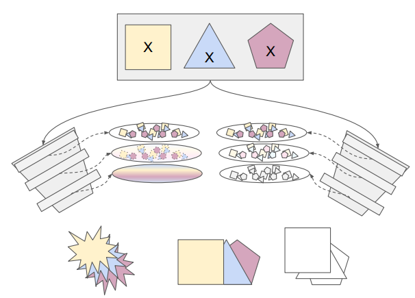
Deep learning models can automatically learn and abstract the complex relationships between input data and output targets, even when those relationships are not obvious or direct at the outset. Deep machine learning models are powerful precisely because they can take arbitrary inputs and learn a mapping to the desired outputs.
Deep Learning in Epidemiology
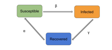
The SIR model divides a population into three categories — Susceptible, Infected, and Recovered — and attempts to define the transitions among them. In the past, identifying these categories and their transitions accurately was extremely difficult.
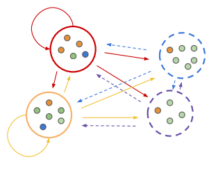
Deep learning has demonstrated its ability to handle exactly this kind of complex disease dynamics and multi-dimensional data — data that traditional compartmental models and statistical models struggle to capture. Deep learning can analyze and understand the intricate patterns of disease transmission, offering a finer-grained and more dynamic analysis of spread than traditional methods.
COVID Modeling
Epidemiological modeling depends on both time and space: tomorrow’s case count depends on yesterday’s case count and on today’s counts among neighbors. It is therefore a multimodal problem — and also a graph problem.
The team models it with a layered graph.
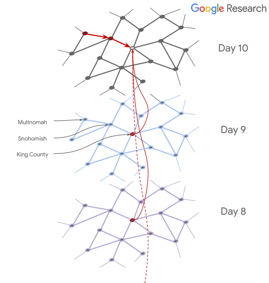
In the figure above, each node represents a particular time and place, and its own features are the case count and internal mobility data.
The graph is modeled as 150 layers, each layer corresponding to one point in time. Edges within a layer capture spatial properties, with weights representing travel distance; edges between layers capture temporal properties, with weights based on the time elapsed between the nodes they connect (the longer the interval, the lower the weight — an inverse relationship).
This design lets the model capture both dynamics over time (through the temporal edges) and connections across space (through the spatial edges), leading to a better understanding and prediction of how COVID-19 spreads.
This example illustrates a broader point: a major advantage of graph data is the ability to bring context into the analysis — when analyzing a node, its surrounding neighbors can serve as additional sources of information.
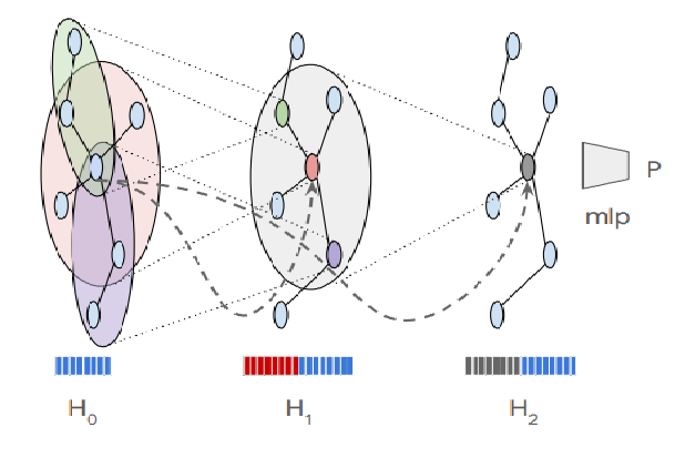
GCNs exploit exactly this: by learning the complex relationships between a node and its neighborhood, they improve both the accuracy and the efficiency of analysis and prediction. Such a model considers not only the attributes of an individual node but also its position in the graph and the influence of the nodes around it.
Privacy-Preserving Computation
Privacy is a fundamental concern when analyzing user data, and graph data (social network graphs, transaction graphs, and so on) is no exception. The talk raises two application scenarios around graph data privacy:
Using graph mining (graph clustering) to improve user privacy: can graph mining techniques, and graph clustering in particular, strengthen user privacy? The key question is whether we can use these techniques to identify and protect the sensitive parts of user data, thereby raising the level of privacy protection.
Protecting user privacy in social network applications: how do we protect user privacy in social network applications? Social graphs typically contain a great deal of sensitive information about personal relationships and interactions. The key question is how to design and implement mechanisms that protect this data from unauthorized access or misuse, while still permitting legitimate and beneficial data analysis and social interaction.
These two scenarios reflect the dual challenge of privacy protection for graph data: on one hand we want to exploit the structure and properties of graph data to strengthen user privacy, and on the other we must ensure the data is not abused and that users are shielded from privacy violations.
On the privacy-preserving computation front, one Google effort is FLoC — Federated Learning of Cohorts.
FLoC
FLoC (Federated Learning of Cohorts) is a privacy-preserving web advertising technology and part of Chrome’s Privacy Sandbox initiative, whose goal is to phase out the use of third-party cookies.
Its basic principle is to take a user’s browsing history as input and replace identifiable third-party cookies with anonymous cookies shared by many users, creating FLoCs (cohorts) that contain at least k users with similar browsing interests. In this way, advertisers can target cohorts with similar interests rather than serving ads based on the specific behavioral data of individual users. This reduces the intrusion on personal privacy while still allowing personalized ad targeting.
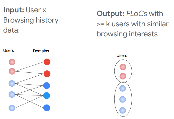
An important question in this project is how to determine cluster size. In other words, the clustering process must ensure that every cluster reaches some minimum size, since individuals are harder to single out within larger clusters.
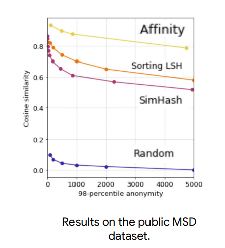
Through experiments, the authors show that Affinity maintains high cosine similarity while also ensuring a high degree of anonymity.
On-Device Public-Private Graph Model
The On-Device Public-Private Graph Model is a model for data processing and analysis in recommender systems. It is designed to perform complex computation on a user’s personal device without leaking the user’s private information. Its focus is on combining public and private data in the computation.
Realizing this model comes down to one question: “Can we keep all private data and contact information on the user’s device, without sacrificing any privacy, and still solve important machine learning problems?”
The approach proposed by the Google team is shown in the figure below.
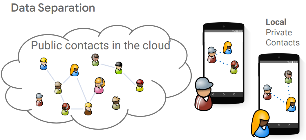
Users can voluntarily choose which portion to keep locally as private data; the non-private portion is uploaded to the cloud and forms the public data available to the server.
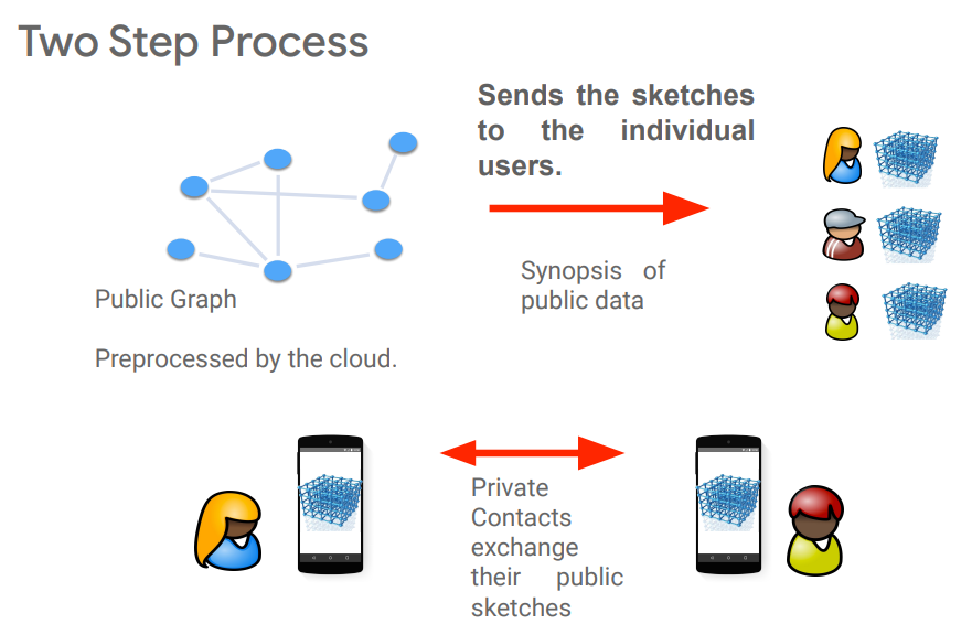
As the figure above shows, the workflow consists of two steps:
- The public data in the cloud sends a summary to individual users.
- Individual users can exchange public data among themselves.
Clustering and Causal Inference
Causal inference is a branch of statistics that attempts to establish cause-and-effect relationships. Its theory is widely applied in randomized experiments such as clinical trials and A/B tests.
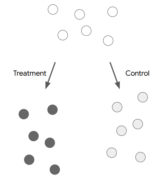
Randomized experiments, however, can suffer from interference: the treatment applied to one subject may affect another. In educational research, for instance, applying a teaching method to a group of students may affect not only those students but also their teachers, their classmates, and the overall learning environment of the school, thereby confounding the results.
To come as close as possible to the “all treated” and “all control” conditions, randomized experiments assign subjects to the treatment or control group by cluster. Returning to the example above: if a study aims to evaluate the effect of an educational intervention that could influence the learning atmosphere of an entire class, the researcher might choose the whole class rather than the individual student as the unit of randomization. That way, all students in a class either receive the intervention or do not, which helps ensure the effect is evaluated at the class level and reduces the problem of interference between individuals.
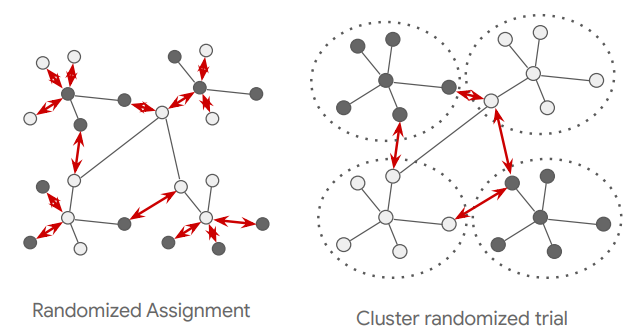
As the figure above shows, if we take individuals as the experimental units, the units influence one another — with more than ten such interactions. To address this, we take clusters as the experimental units instead. As shown on the right, in that example the number of interactions drops to just four.