Paper Review | Emergent Abilities of LLMs Are a Mirage

Title: Are Emergent Abilities of Large Language Models a Mirage?
Institution: Computer Science, Stanford University
Authors: Rylan Schaeffer, Brando Miranda, Sanmi Koyejo
Arxiv Link: https://arxiv.org/abs/2304.15004
Comments: NeurIPS 2023
Date: 2023.04.28
Preface
This paper was posted on arXiv on April 28, 2023. Two versions later, it won a Best Paper award in the main track at NeurIPS 2023 (2 out of 3584).
Emergent Abilities
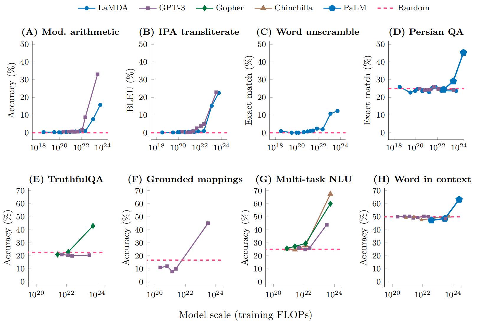
The paper notes that a great deal of work claims LLMs display abilities that are absent at smaller scales but present at larger ones — what people commonly call emergent abilities, or emergence.
An “emergent ability” is a capability or behavior that a model displays only once it becomes large enough, one that smaller models did not have — a metric that suddenly shoots up, for instance.
As the figure above shows, for model families such as LaMDA and GPT-3, accuracy jumps abruptly once the parameter count crosses a certain critical point. That is emergence.
Emergent abilities have two defining features:
- Sharpness: an abrupt rise as the parameter count increases linearly
- Unpredictability: they appear suddenly at some uncertain critical parameter count
Does Emergence Really Exist?
To give away the conclusion: this paper shows that LLMs exhibit no genuine “emergence”; their capabilities grow smoothly as parameters increase.
Emergence is not a product of growth in a model’s parameter count. It is an illusion created by the metric the researcher happened to choose.
The authors’ starting point is that the metrics previously used to measure model capability are discrete rather than linear, and that this is what produces apparent emergence. So what happens if we swap in a linear or continuous metric instead — does a model’s capability turn out to be smooth, continuous, and predictable?
Explaining Emergent Abilities
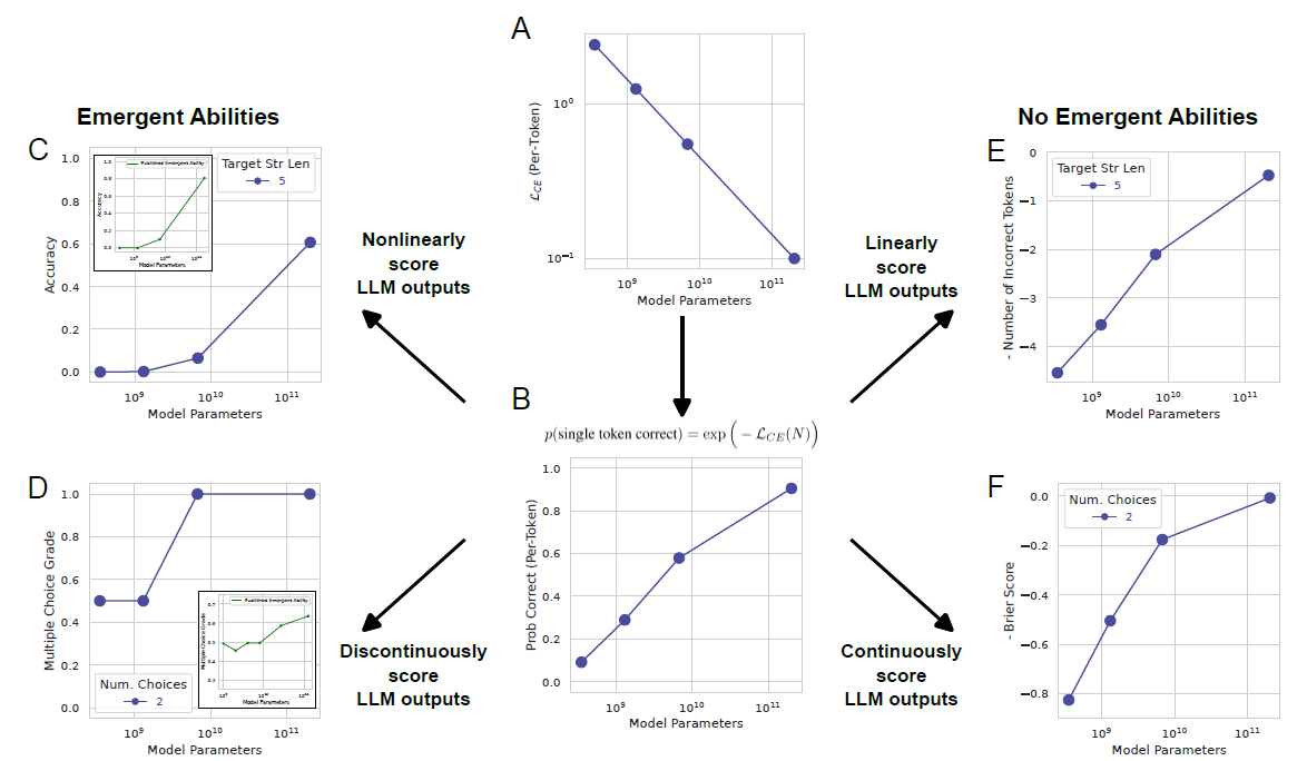
The authors open with a question of their own: how can a smooth, continuous, predictable change in model performance be made to look abrupt and unpredictable? Their answer is that a researcher’s choice of a nonlinear or discontinuous metric can distort how the model’s performance appears, making it seem to change abruptly and unpredictably.
Experience tells us that a neural network’s capability scales in a fixed proportion with the amount of training data, the parameter count, and the compute expended. Taking that as given, assume the following holds (Figure 2.A): $$ \mathcal{L}_{CE}(N)=\left(\frac Nc\right)^\alpha $$ where $L_CE$ denotes cross entropy, $N$ denotes the parameter count, and $c>0$ and $\alpha<0$ are constants. In practice, cross entropy is defined as: $$ \mathcal{L}_{CE}(N)\overset{\mathrm{def}}{\operatorname*{=}}-\sum_{v\in V}p(v)\log\hat{p}_N(v) $$ This formula measures the discrepancy between the model’s predicted distribution $\hat{p}_N$ over the whole vocabulary $V$ and the true distribution $p$. For each possible token $v$, the true distribution $p(v)$ gives the true probability that token $v$ occurs, while $\hat{p}_N(v)$ is the probability the model assigns to token $v$.
Since $p(v) = 0$ for all $v \neq v^*$ and $p(v^*) = 1$, only the term with $v = v^*$ survives the sum, and the formula simplifies to:
$$ \mathcal{L}_{CE}(N)=-\log\hat{p}_N(v^*) $$
The probability that each token is predicted correctly is (Figure 2.B): $$ \begin{align*} p(\text{single token correct})& =\exp\left(-\mathcal{L}_{CE}(N)\right)\\ & =\exp\left(-(N/c)^\alpha\right) \end{align*} $$ Now suppose the researcher chooses a metric that requires $L$ tokens to all be correct. The task might be, for example, $L$-digit integer addition, scoring $1$ if all $L$ output digits match the target digits exactly, with no insertions, deletions, or substitutions, and $0$ otherwise. If each token’s correctness is independent, the probability of scoring $1$ is: $$ \begin{align*} \operatorname{Accuracy}(N) &\approx p_N\left(\text{single token correct}\right)^\text{num. of tokens} \\ &= \exp\left(-(N/c)^\alpha\right)^L \end{align*} $$
$$\text{Exact String Match}\stackrel{\text{def}}{=}\begin{cases}1&\text{if output string exactly matches target string}\\0&\text{otherwise}\end{cases}$$
This choice of metric makes performance scale nonlinearly with the length of the token sequence. Plotting performance on a linear-log axis (Figure 2.C) reveals abrupt, unpredictable jumps on longer sequences — a very close match to the emergent abilities other researchers have claimed.
And what happens if we use a linear metric such as Token Edit Distance? $$ \begin{aligned} \text{Token Edit Distance}(N) &\approx L(1-p_N(\text{single token correct})) \\ &= L\left(1-\exp\left(-(N/c)^\alpha\right)\right) \end{aligned} $$ When model capability is measured with the linear metric Token Edit Distance, it becomes smooth, continuous, and predictable (Figure 2.E).
“Token Edit Distance” is a way of measuring the difference between two sequences. It counts the minimum number of edit operations — insertions, deletions, and substitutions of a single token — needed to turn one sequence into the other. In this context, a “token” usually means a word, a character, or another linguistic unit.
For example, if we have two sequences, sequence A being “cat” and sequence B being “bat”, the token edit distance from A to B is 1, since we need only substitute “b” for “c”.
If the discrete metric Multiple Choice Grade is used, emergence is observed (Figure 2.D), but if the continuous metric Brier Score is used, emergence disappears (Figure 2.F).
Multiple Choice Grade:
$$\\ \text{Multiple Choice Grade}\stackrel{\text{def}}{=}\begin{cases}1&\text{if highest probability mass on correct option}\\0&\text{otherwise}\end{cases}$$Brier Score: $$ BS = \frac{1}{N} \sum_{i=1}^{N} (f_i - o_i)^2$$ where:
- $N$ is the number of predictions.
- $f_i$ is the predicted probability of occurrence for the $i$-th prediction (the probability output by the model).
- $o_i$ is the observed value of the actual outcome for the $i$-th case (usually 1 if the event occurred and 0 if it did not).
As an example, suppose you are predicting whether football matches will end in a draw. For three matches, your model predicts draw probabilities of 0.3, 0.6, and 0.2. The actual outcomes are that the first match was a draw (1) while the second and third were not (0).
The Brier Score is then computed as follows:
- For the first match, the prediction error is $ (0.3 - 1)^2 = 0.49 $.
- For the second match, the prediction error is $ (0.6 - 0)^2 = 0.36 $.
- For the third match, the prediction error is $ (0.2 - 0)^2 = 0.04 $. The Brier Score is the average of these errors, so in this example it is $ \frac{0.49 + 0.36 + 0.04}{3} = 0.2967 $.
In summary, the illusion of emergence has two causes.
- The metrics adopted by earlier work are discrete rather than continuous or linear, and that is what gives rise to the appearance of emergence.
- Earlier work experimented only over a narrow range of parameter counts. Model sizes are typically 6B, 7B, 13B, 33B, 70B and so on, which cover only a handful of points in the range. Had sizes such as 6B, 6.1B, 6.2B, 6.3B … 70.1B, 70.2B been available, people would have seen that discrete metrics relate to parameter count exponentially rather than by a sudden jump.
This work fully deserves its Best Paper award at NeurIPS 2023. Its starting point is simple, yet its insights are far-reaching, creative, and genuinely illuminating. Before it appeared, emergence had become a widely accepted “magical phenomenon” in the field, and a good deal of research had been devoted to it, probing experiments included. Against that backdrop, the paper works from the details up to show that “emergence” does not actually exist — an eye-opening result for many researchers, this author among them.